NEURAL NETWORKS
TERM PROJECT
CHARACTER RECOGNATION
INTRODUCTION
One of the most classical applications of the Artificial Neural Network is the Character Recognition System. This system is the base for many different types of applications in various fields, many of which we use in our daily lives. Cost effective and less time consuming, businesses, post offices, banks, security systems, and even the field of robotics employ this system as the base of their operations. Wither you are processing a check, performing an eye/face scan at the airport entrance, or teaching a robot to pick up and object, you are employing the system of Character Recognition.
One field that has developed from Character Recognition is Optical Character Recognition (OCR). OCR is used widely today in the post offices, banks, airports, airline offices, and businesses. Address readers sort incoming and outgoing mail, check readers in banks capture images of checks for processing, airline ticket and passport readers are used for various purposes from accounting for passenger revenues to checking database records, and form readers are used to read and process up to 5,800 forms per hour. OCR software is also used in scanners and faxes that allow the user to turn graphic images of text into editable documents. Newer applications have even expanded outside the limitations of just characters. Eye, face, and fingerprint scans used in high-security areas employ a newer kind of recognition. More and more assembly lines are becoming equipped with robots scanning the gears that pass underneath for faults, and it has been applied in the field of robotics to allow robots to detect edges, shapes, and colors.
Optical Character Recognition has even advanced into a newer field – Handwritten Recognition, which of course is also based on the simplicity of Character Recognition. The new idea for computers, such as Microsoft’s new Tablet Pc, is pen-based computing, which employs lazy recognition that runs the character recognition system silently in the background instead of in real time.
1. Creating the Character Recognition System
The Character Recognition System must first be created through a few simple steps in order to prepare it for presentation into MATLAB. The matrixes of each letter of the alphabet must be created along with the network structure. In addition, one must understand how to pull the Binary Input Code from the matrix, and how to interpret the Binary Output Code, which the computer ultimately produces.
2. Character Matrixes
A character matrix is an array of black and white pixels; the vector of 1 represented by black, and 0 by white. They are created manually by the user, in whatever size or font imaginable; in addition, multiple fonts of the same alphabet may even be used under separate training sessions.
3. Creating a Character Matrix
First, in order to endow a computer with the ability to recognize characters, we must first create those characters. The first thing to think about when creating a matrix is the size that will be used. Too small and all the letters may not be able to be created, especially if you want to use two different fonts. On the other hand, if the size of the matrix is very big, their may be a few problems: Despite the fact that the speed of computers double every third year, their may not be enough processing power currently available to run in real time.
Training may take days, and results may take hours. In addition, the computer’s memory may not be able to handle enough neurons in the hidden layer needed to efficient and accurately process the information. However, the number of neurons may just simply be reduced, but this in turn may greatly increase the chance for error. A large matrix size of 20 x 20 was created, through the steps as explained above, because it may not be able to process in real time. (See Figure 1) Insteadof waiting a few more years until computers have again increased in their processing speed, another solution has been presented which will be explained fully at the end of this paper.
4. Neural Network
The network receives the 400 Boolean values as a 400-element input vector. It is then required to identify the letter by responding with a 26-element output vector. The 26 elements of the output vector each represent a letter. To operate correctly, the network should respond with a 1 in the position of the letter being presented to the network.
All other values in the output vector should be 0. In addition, the network should be able to handle noise. In practice, the network does not receive a perfect Boolean vector as input. Specifically, the network should make as few mistakes as possible when classifying vectors with noise of mean 0 and standard deviation of 0.2 or less.
5. Architecture
The neural network needs 400 inputs and 26 neurons in its output layer to identify the letters. The network is a two-layer log-sigmoid/log-sigmoid network. The log-sigmoid transfer function was picked because its output range (0 to 1) is perfect for learning to output Boolean values. The hidden (first) layer has 52 neurons. This number was picked by guesswork and experience. If the network has trouble learning, then neurons can be added to this layer.
The network is trained to output a 1 in the correct position of the output vector and to fill the rest of the output vector with 0’s. However, noisy input vectors may result in the network not creating perfect 1’s and 0’s. After the network is trained the output is passed through the competitive transfer function compet. This makes sure that the output corresponding to the letter most like the noisy input vector takes on a value of 1, and all others have a value of 0. The result of this post-processing is the output that is actually used.
6. Setting the Weights
There are two sets of weights; input-hidden layer weights and hidden-output layer weights. These weights represent the memory of the neural network, where final training weights can be used when running the network.
Initial weights are generated randomly there, after; weights are updated using the error (difference) between the actual output of the network and the desired (target) output. Weight updating occurs each iteration, and the network learns while iterating repeatedly until a net minimum error value is achieved. First we must define notion for the patterns to be stored Pattern p. a vector of 0/1 usually binary– valued. Additional layers of weights may be added but the additional layers are unable to adopt. Inputs arrive from the left and each incoming interconnection has an associated weight, wji. The perception processing unit performs a weighted sum at its input value.
Weights associated with each inter connection are adjusted during learning .The weight to unit J from unit j from unit I is denoted as wi after learning is completed the weights are fixed from 0 to 1. There is a matrix of weight values that corresponds to each layer at inter connections
7. Training
To create a network that can handle noisy input vectors it is best to train the network on both ideal and noisy vectors. To do this, the network is first trained on ideal vectors until it has a low sumsquared error. Then, the network is trained on all sets of ideal and noisy vectors. The network is trained on two copies of the noise-free alphabet at the same time as it is trained on noisy vectors. The two copies of the noise-free alphabet are used to maintain the network’s ability to classify ideal input vectors. Unfortunately, after the training described above the network may have learned to classify some difficult noisy vectors at the expense of properly classifying a noise-free vector. Therefore, the network is again trained on just ideal vectors.
This ensures that the network responds perfectly when presented with an ideal letter. All training is done using backpropagation with both adaptive learning rate and momentum with the function trainbpx.
8. System Performance and Results
The reliability of the neural network pattern recognition system is measured by testing the network with hundreds of input vectors with varying quantities of noise. The script file appcr1 tests the network at various noise levels, and then graphs the percentage of network errors versus noise. Noise with a mean of 0 and a standard deviation from 0 to 0.5 is added to input vectors. At each noise level, 100 presentations of different noisy versions of each letter are made and the network’s output is calculated.
The output is then passed through the competitive transfer function so that only one of the 26 outputs (representing the letters of the alphabet), has a value of 1. The above input was trained, and tested with the following specifications.
CONCLUSION
This problem demonstrates how a simple pattern recognition system can be designed. Note that the training process did not consist of a single call to a training function. Instead, the network was trained several times on various input vectors. In this case, training a network on different sets of noisy vectors forced the network to learn how to deal with noise, a common problem in the real world.
Despite variations in character size, orientation, and position, the neural network was still able to recognize many of the characters. Combined with stroke analysis and temporal information, neural networks look to be a very promising solution. This has resulted in some researchers advocating ‘lazy recognition’, not attempting to do character recognition in real time.
REFERENCES
1. Pratt, William K. Digital Image Processing. New York: John Wiley & Sons, Inc., 1991. p. 634.
2. Horn, Berthold P. K., Robot Vision. New York: McGraw-Hill, 1986. pp. 73-77.
3. Pratt, William K. Digital Image Processing. New York: John Wiley & Sons, Inc., 1991. p. 633.
4. Haralick, Robert M., and Linda G. Shapiro. Computer and Robot Vision, Volume I. Addison-Wesley, 1992.
5. Ardeshir Goshtasby, Piecewise linear mapping functions for image registration, Pattern Recognition, Vol 19, pp. 459-466, 1986.
6. Ardeshir Goshtasby, Image registration by local approximation methods, Image and Vision Computing, Vol 6, p. 255-261, 1988.
7. Jain, Anil K. Fundamentals of Digital Image Processing. Englewood Cliffs, NJ: Prentice Hall, 1989. pp. 150-153.
8. Pennebaker, William B., and Joan L. Mitchell. JPEG: Still Image Data Compression Standard. Van Nostrand Reinhold, 1993.
9. Gonzalez, Rafael C., and Richard E. Woods. Digital Image Processing. Addison-Wesley, 1992. p. 518.
10. Haralick, Robert M., and Linda G. Shapiro. Computer and Robot Vision, Volume I. Addison-Wesley, 1992. p. 158.
11. Floyd, R. W. and L. Steinberg. “An Adaptive Algorithm for Spatial Gray Scale,” International Symposium Digest of Technical Papers. Society for Information Displays, 1975. p. 36.
12. Lim, Jae S. Two-Dimensional Signal and Image Processing. Englewood Cliffs, NJ: Prentice Hall, 1990. pp. 469-476.
13. Canny, John. “A Computational Approach to Edge Detection,” IEEE Transactions on Pattern Analysis and Machine Intelligence, 1986. Vol. PAMI-8, No. 6, pp. 679-698.
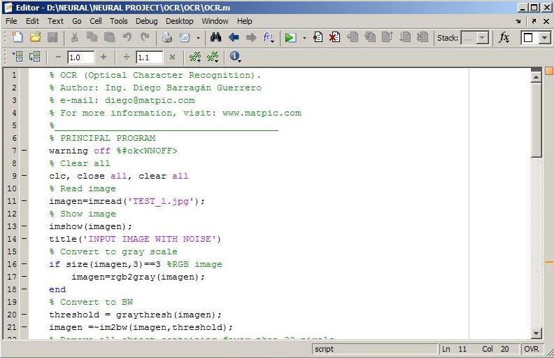
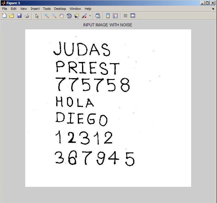
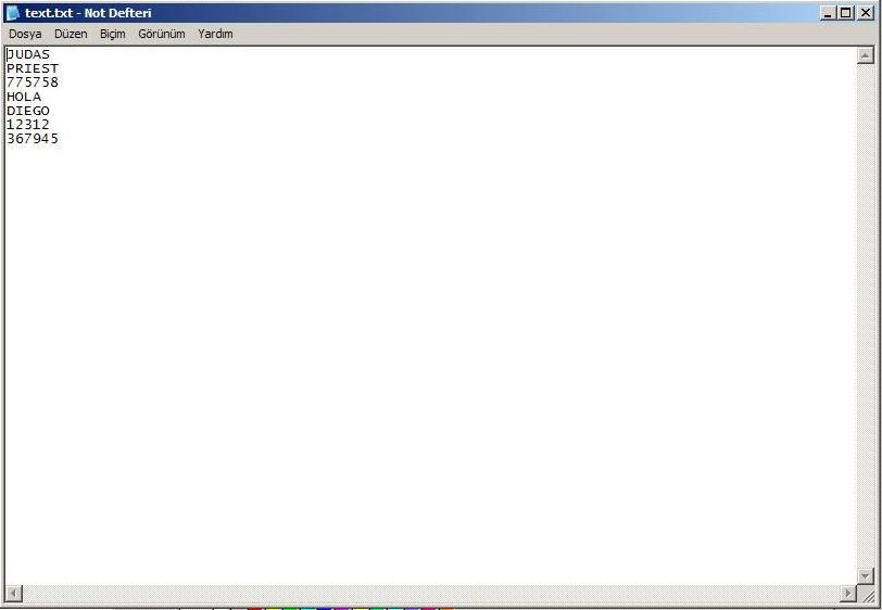
SHOW DEMO IN THE MATLAB (WITH PICTURE)
STEP1 : Run the program in the Matlap
STEP2 : Program takeing image
STEP3 : And write character include txt file.


